As you may have learnt in PM Course 1, project planning and tracking are determined by the deadlines set by your clients and the number of steps in a project.
You should remember that every project is unique and so each project might require different or new resources.
For accurate planning, you will have to use standard units for measuring the workload.
In our example, we will use the following scheme:
- Translation: 2,500 words/day
- Revision: between 5,000 and 7,500 words/day
- Reviewing: between 10,000 and 20,000 words/day
- DTP – Word: 8 pages/hour
- Illustrations: 3-4 illustrations/hour
So, you can calculate the time required per task on the basis of the volume of the project as a whole.
2.1.1 Insert Data Manually
Let's take the example of creating a planning table for a small project consisting of:
- 15,000 words of text (translation, revision and reviewing in one target language only)
- 50 pages in MS Word for DTP.
The information you need is:
- the total number of units
- the number of units achievable per hour or per day.
Make sure you use realistic unit calculations, such as a working day consisting of eight working hours and a week of five working days. Permissible or acceptable working hours may vary from country to country. According to the unit/time scheme on the previous page, this workload requires a total of 10.5 working days – 6 days for translation, 1.5 day for revision, 1 day to review, 1 day DTP and final proofreading, and 1.5 day for sending and receiving materials and feedback from the client and setting up the project.
Remember that these steps will not necessarily be performed one after the other. It is part of the art of planning process to get all tasks completed in the shortest elapsed time.
So the tasks will not be planned to occur consecutively, but to overlap and run partly in parallel. In our example, there is a team of 2 translators, 1 reviser, 1 reviewer, 1 DTP specialist and 1 person for final proofreading. Furthermore, there are processes going in parallel.
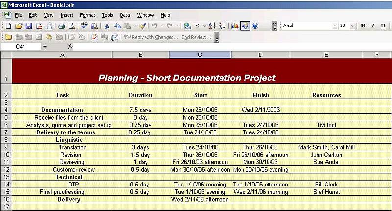 Translation Project Planning
2.1.2 Insert Data Automatically
This feature is very helpful if you want to insert data from a different file in the current spreadsheet . By using Data|Import External Data, you will be able to import data from external files (.mdb, .txt, .doc, etc.) into your open .xls.
A chart like this one will help you visualise the progression and planning for each task. You could use a different colour for every task, or to distinguish completed and on-going tasks.
To change the colour of selected cells, click on the Fill Color icon and choose the desired colour.
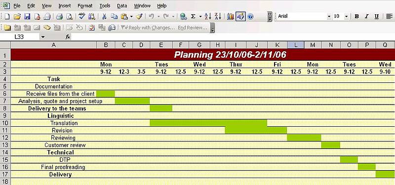 Colour-coded Planning
As you saw previously, the workplan will be shown and explained to the client.
Besides creating charts for planning, you can create other charts for the resources, inputs and outputs needed for each task.
 Task Planning 1/2
Colour-coding can be used to illustrate the status of tasks. For example:
- black – finished
- red – on-going
- green – not started
 Task Planning 2/2
Talking about planning and the granularity of a translation project workflow, Istvan Lengyel brings in the notion of building blocks(MultiLingual Computing, #84, December 2006).
According to this metaphor, for every task identified there is a corresponding building block. Each building block must comprise all the resources needed for its completion. By using this kind of granular planning, one can measure and foresee the impact that the non-realisation, delay or change of one building block will have on the rest of the project.
For example, for the proofreading task, he identifies the following blocks: Bilingual text(s) (xx-yy), Updated termbase, Translation brief, Proofreader and Target document(s).
As we have already seen, the advantage of creating such blocks is in planning all the resources necessary for each task and possibly preventing some problems that might otherwise appear in the life of a project.
In Excel, this can be easily achieved by creating one worksheet for every building block and using colour coding to reflect the stage of completion of each one.
The Insert Function... feature of Excel is extremely useful. It allows you to create formulas that perform mathematical functions (addition, subtraction, division, etc.) on data from the same worksheet or from different worksheets within a workbook.
In the example below, we create an invoice for a new project.
Client: Cosmo Translation Company
Source language: English
Target languages: French and Italian
Project description:
- User manual in MS Word - 125,000 words and 105 screenshots
- DTP - approximately 200 words per page
- Software requirements -Trados
- French:
- 30% perfect matches
- 30% new words
- 40% fuzzy matches (from 75 to 99%)
- Italian:
- 17% perfect matches
- 53% new words
- 30% fuzzy matches (from 75 to 99%)
- 10% for project management
The invoice sections can be created per task or per language, as illustrated below.
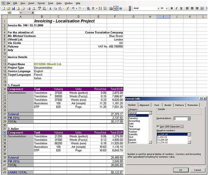
Creating an Invoice

You can format the cells containing prices as numbers with two decimal places (Format|Cells). Make sure you and your client understand which separators are being used - 1,000 has different meanings in the UK and in France.
The values in column F are obtained through formulas. In this project, for French, there are 125,000 words, out of which –
- 30% perfect matches
- 30% new words
- 40% fuzzy matches (from 75 to 99%)
So, cell C21 = 0.3*125,000, C22 = 0.4*125,000 and C23 = 0.3*125,000.
Also, C25 = 125,000/200, since DTP is priced at 200 words per page.
Two of the values in the Price/Unit are obtained through formulas:
- the perfect match price represents one third of the new word price, so, E21 = E23/3
- the fuzzy match price represents two thirds of the new word price, so, E22 = E23/3*2
The Total EUR column is obtained as follows:
- F21 = C21*E21 - the total price for French perfect matches.
- If you copy this formula into the next four cells in the column, they will be automatically updated using the data from the relevant cells (in this case: F22 = C22*E22 ... F25 = C25*E25). You can also manually input each of these formulas.
- F27 = SUM(F21:F26) - the sum of the values from the cells in the range F21-F26. To edit this formula go to Insert|Function|SUM and select (with the mouse) the cells whose values are to be added.
- F28 = 0.1*F27 (10% for project management).
- F29 = SUM(F27:F28) - the total sum for French tasks.
The same is done for Italian and then the two are added together in the Grand Total.
As we saw previously, the gross profit margin is defined as "the difference between the selling price of an item and the purchase or manufacturing cost, expressed as a percentage of the selling price". This number represents the percentage of the revenue that a company retains after paying for the basic costs of production.
This percentage is obtained after having deducted the variable costs of the project. From the gross profit margin, the fixed costs are then deducted and the result is the net profit margin.
The gross profit margin is calculated using the following formula:
Gross Profit Margin in % = (Sales – Costs)/ Sales
You can easily calculate it by using simple formulas in Excel.
Examples for two different projects:
For the first project, you know the sales and costs figures, so the gross profit margin (GP Margin) is…
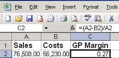
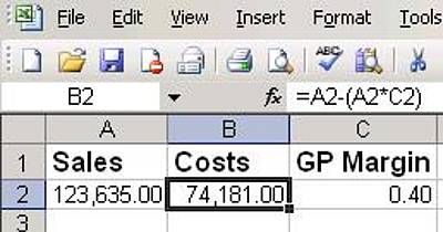
For the second project, you know the sales figure and the gross profit margin, so you can calculate the maximum costs figure.
You might want to do this calculation in the middle of a project when you know the price agreed with your client (Sales) and you also know the minimum GP Margin you can have. This can happen, for example, when you have to squeeze in a task you did not foresee at the beginning of the project, and hence did not budget for it.
The result of this calculation will tell you the maximum Costs that you can afford while keeping the project profitable.
To read more about this, go to the eCoLoTrain LTC Organiser course.
Display currency symbol
Another important feature of Excel, especially for creating quotes and purchase orders, is to change or display the currency symbol.
To customise the currency symbol, go to Format|Cells. Under the Number tab, click Currency and in the Symbol box, click the currency symbol that you want.
To display a number with the default currency symbol, select the cell or range of cells and then click the Currency Style icon on the Formatting toolbar or go to Format|Style and in the Style name drop-down menu choose currency. Make sure the Number box is selected and click OK.
Other formulas
Other formulas can be found in the Insert|Function menu, such as:
- AVERAGE(number1;number2;…) calculates the arithmetical average of the values stored within the selected cells
- IF(logical_test; value_if_true; value_if_false) - checks whether a condition provided inside the logical_test is met, and returns one value if TRUE and another value if FALSE. Example: IF(F29>F41; F29; F41) = 28,008.75. This particular test returns the larger of two values.
- MAX(number1; number2;…) returns the largest value in a set of values - Example: MAX(F20:F41) = 28,008.75
- MIN(number1; number2;…) - returns the smallest value in the indicated set; ignores the logical values and text
- HYPERLINK(link_location; friendly_name) - creates a hyperlink that opens a document stored on the local computer, on a network server, or on the Internet - Example HYPERLINK(https://ecolotrain.uni-mainz.de/de/)
- Days360 – returns the number of days, between two dates, based on a 360-day year
- Logical - logical functions (could be used inside the formulas), returning TRUE or FALSE. Examples: AND, IF, NOT, OR

